Overview

PEPIS is a pipeline that is dedicatedly developed for Polygenic, specifically, Epistatic QTL mapping. Commonly, the user upload their coded genotypic data and phenotypic data, then the kinship matrices, polygenic components' ratio, and comprehensive LRT based QTL mapping to the target quantitative trait can be calculated, analyzed and estimated. The results from PEPIS can help breeders to understand the genetic mechanisms of complex quantitative trait, such as yield, weight, etc., and then develop the more efficient breeding programs.

Pipeline Flowchart

The whole pipeline include two sequential sub-pipelines: Pipeline 1 is responsible for the calculating and outputting the kinship matrices based on the user-uploaded genotypic data files, while pipeline 2, based on the inputting trait related genotypic data and the outputting kinship matrices from pipeline 1, is responsible for estimating the polygenic components' contribution to the specific trait, and the 1D/2D LRT(Likelihood Ratio Test) profiles for main(additive, dominance)/epistatic(aa, ad, da, dd) genetic effects. Additionally, the Kinship matrix calculation and epistatic QTL mapping need more calculations, and implemented in parallel structures. Fig.1 gives the pipeline flowchart of PEPIS.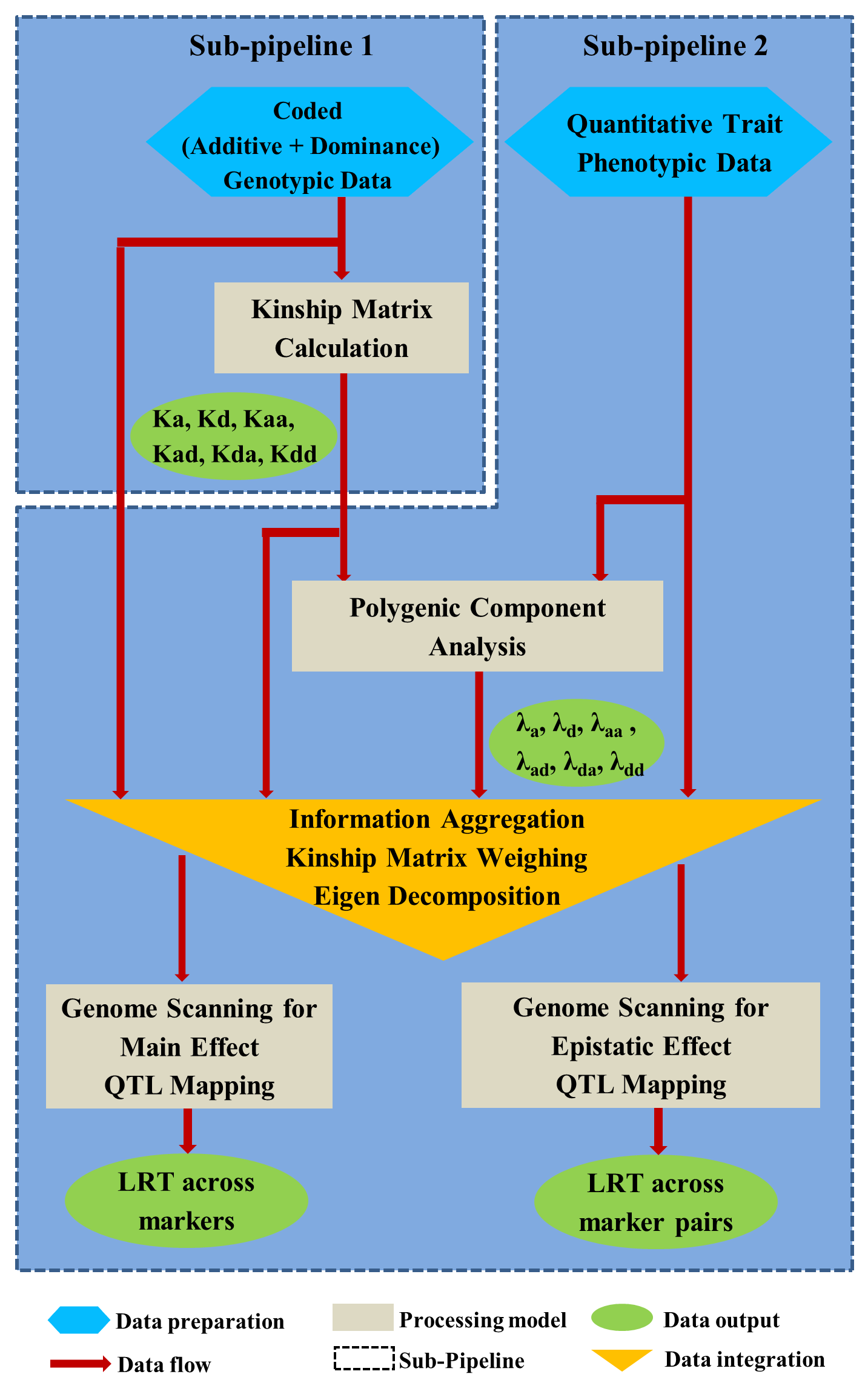

Fig. 1 Pipeline Flowchart of PEPIS for Polygenic QTL Mapping

Representative Case Applications for Kinship Matrix Calculation

At least one of the genotypic(additive or dominance) files is needed. If the encode of [-1,0,+1] is adopted for additive genotype and the encode of [0,1,0] is adopted for dominance genotype, PEPIS support the function to retrieve the complete dominance genetic information from additive genetic information, only if the user click the option of Z->W Transition. Considering the high calculation burden of epistatic effect, the pipeline also support to calculate all of the 6 kinship matrices(Ka, kd, kaa, Kad, Kda, Kdd) or only the main effect kinship matrix(Ka, kd), if the user click the option of Epistatic Effect. So, there are usually 3 cases to run the pipeline in application

Case 1: Both the additive and dominance genotypic data files are provided, all the 6 kinship matrices or only the 2 main effect kinship matrices can be calculated according to click the option of Epistatic Effect or not.

Case 2: Only the additive genotypic data file is provided, all the 6 kinship matrices, or the 2 main effect kinship matrices, or additive together with its' related epistatic kinship matrix (Ka, Kaa), or only the additive main effect kinship matrix(Ka) can be calculated according to click the combinational option of Epistatic Effect and/or Z->W Transition.

Case 3: Only the dominance genotypic data file is provided, the dominance together its' epistatic kinship matrix (Kd, Kdd) or only the dominance main effect kinship matrix(Kd) can be calculated according to click the option of Epistatic Effect or not.

Representative Case Applications for Polygenic QTL Mapping

Logically, if the Pipeline 1 can generate the 6 complete kinship matrices, the 6 polygenic components can be analyzed. Further, if both the additive and dominance genotypic data files are provided, then, one or both of the main effect and epistatic QTL mapping can be calculated

Case 1: Both the additive and dominance genotypic data files are provided, all the 6 kinship matrices can be calculated; Using the provided phenotypic data file, the polygenic components can be analyzed, further, the main and epistatic QTL mapping can estimated according to user's need.

Case 2: Only the additive genotypic data file is provided, all the 6 kinship matrices can be calculated; Using the provided phenotypic data file, the polygenic components can be analyzed, but the QTL mapping can't be implemented.

File Format and Requirements for Genotypic and Phenotypic Data

The inputting genotypic and Phenotypic data file(s) are text file(s) and delimited by comma. All of the genotypic information in the files must be strictly stored as a format of m rows/lines and n columns (absolute no head or other supporting information), where m and n corresponds to the number of SNP marker/bin, and population individuals respectively. The phenotypic data file is stored as a vector with one column and n rows. The user needs to modify the format of their genotypic and phenotypic files according to the provided additive genotypic example file , dominance genotypic example file, and Phenotypic example file with the marker number m=1619 and individual number n=278.

QTL Mapping Results from PEPIS and its Biological Explanation

Once the pipeline2 finished, a text file for the polygenic component ratio to the target trait will be outputted. Additionally, if any of the main effect and epistatic effect QTL mapping is checked, the LRT based QTL mapping that corresponding to the text files for the trait related LRT across all the SNP markers(bins) or marker pairs will be outputted. Based on the polygenic component analysis result file, the polygenic component ratio can be displayed, which can provide a big picture of genetic structure for the quantitative trait. Fig.2 provides a pie chart for the polygenic component ratio to the target traits.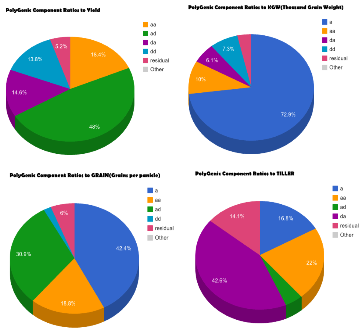

Fig. 2 Polygenic component ratio to the quantitative traits of YIELD, KGW(thousand grain weight), GRAIN(Grain per panicle) and TILLER.

Based on the LRT outputted files, A LRT profile across the whole genome can be generated, which can provide a comprehensive genetic mechanism for some complex trait. Note, the main effect LRT is 1D LRT across all SNP/markers while the epistatic LRT is a 2D LRT for marker pairs. Fig.3 provide a the 1D main effect related LRT profiles for 4 different traits across the SNP/Bin markers in the whole genome(the vertical dash lines pinpoints the regions of 12 chromosomes along all the 1619 SNP/Bin markers), and Fig.4 provide the 2D epistatic effect related LRT profiles for the 4 different traits across all 1619*1618/2 SNP/Bin marker pairs in the whole genome.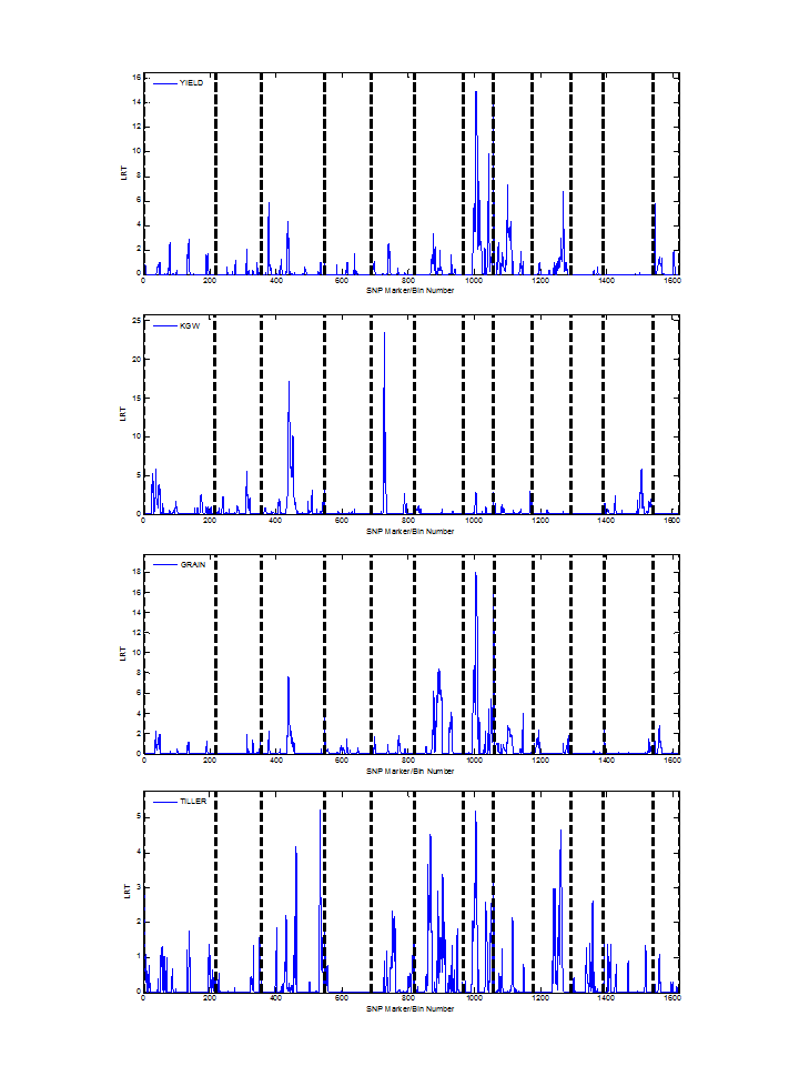

Fig. 3 Illustration of LRT profiles for different traits across the SNP/Bin markers in the whole genome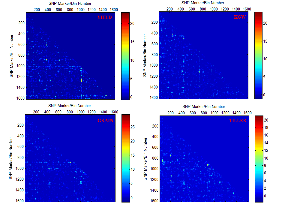

Fig. 4 Illustration of LRT profiles for different traits across the SNP/Bin marker pairs in the whole genome

Reference:

1. Xu, S., Mapping Quantitative Trait Loci by Controlling Polygenic Background Effects. Genetics, 2013. 195(4):p.1709-23.

2. Zhang W, Dai X, Wang Q, Xu S, Zhao PX, PEPIS: A Pipeline for Estimating Epistatic Effects in Quantitative Trait Locus Mapping and Genome-Wide Association Studies, 2016. PLoS Comput Biol, 12(5).